Difficult to pick a favourite out of this lot:
But while simulation is a bit problematic – though immensely entertaining – in football and other sports, it has a totally different meaning in the context of Statistics, and proves to be an essential part of the statistician’s toolbox.
Here’s how it works: at its heart a statistical model describes a process in terms of probabilities. Since computers can be tricked to mimic randomness, this means that in many circumstances they can be used to simulate the process of generating new ‘data’ from the statistical model. These data can then, in turn, be used to learn something about the behaviour of the model itself.
Let’s look at a simple example.
The standard statistical model for a sequence of coin tosses is that each toss of the coin is independent from all others, and that in each toss ‘heads’ or ‘tails’ will each occur with the same probability of 0.5. The code in the following R console will simulate the tossing of 100 coins, print and tabulate the results, and show a simple bar chart of the counts. Just press the ‘Run’ button to activate the code, then toggle between the windows to see the printed and graphical output. Since it’s a simulation you’re likely to get different results if you repeat the exercise. (Just like if you really tossed 100 coins, you’d probably get different results if you did it again.)
[datacamp_exercise lang=”r” height=”500″ max-height=”500″]
[datacamp_pre_exercise_code]
runs<-function(ntoss,nrep,p_head=0.5){
tosses<-sample(c(‘Heads’,’Tails’), size=nrep*ntoss, replace=T, prob=c(p_head,1-p_head))
tosses<-matrix(tosses,nrow=nrep)
l<-apply(tosses,1,function(x)max(rle(x)$length))
hist(l,breaks=(min(l)-.5):(max(l)+.5),col=”lightblue”,main=”Maximum Run Length “,xlab=”Length”)
}
[/datacamp_pre_exercise_code]
[datacamp_sample_code]
#specify number of tosses
ntoss<-100
#do the simulation
tosses<-sample(c(‘Heads’, ‘Tails’), size=ntoss, replace=TRUE)
#show the simulated coins
print(tosses)
#tabulate results
tab<-table(tosses)
#show table of results
print(tab)
#draw barplot of results
barplot(tab, col=”lightblue”, ylab=”Count”)
[/datacamp_sample_code]
[datacamp_solution]
[/datacamp_solution]
[datacamp_sct]
[/datacamp_sct]
[datacamp_hint]
[/datacamp_hint]
[/datacamp_exercise]
That’s perhaps not very interesting, since it’s kind of obvious that we’d expect a near 50/50 split of heads and tails each time we repeat the experiment. But suppose instead we’re interested in runs of heads or tails, and in particular, the longest run of heads or tails in the sequence of 100 tosses. Some of you may remember we did something like this as an experiment at an offsite some years ago. This is sort of relevant to Smartodds since if we make a sequence of 50/50 bets, looking at the longest run of heads or tails is equivalent to looking at the longest run of winning or losing bets. Anyway, the mathematics to calculate the probability of (say) a run of 10 heads or tails occurring is not completely straightforward. But, we can simulate the tossing of 100 coins many times and see how often we get a run of 10. And if we simulate often enough we can get a good estimate of the probability. So, lets try tossing a coin 100 times, count the longest sequence of heads or tails, and repeat that exercise 10,000 times. I’ve already written the code for that. You just have to toggle to the R console window and write
runs(100, 10000)
followed by ‘return’. You should get a picture like this
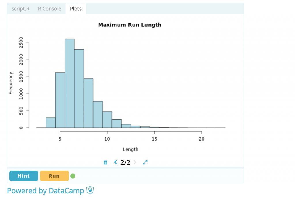
Yours will be slightly different because your simulated tosses will be different from mine, but since we are both simulating many times (10,000 repetitions) the overall picture should be very similar. Anyway, on this basis, I got a run of 10 heads or tails around 400 times (though I could have tabulated the results to get the number more precisely). Since this was achieved in 10,000 simulations, it follows that the probability of a maximum sequence of 10 heads or tails is around 400/10000 = 0.04 or 4%.
Some comments:
- This illustrates exactly the procedure we adopt for making predictions from some of our models. Not so much deadball models, from which it’s usually easy to get predictions by a simple formula, but our in running models often require us to simulate the goals (or points) in a game, and to repeat the game many times, in order to get the probability of a certain number of goals/points.
- You can increase the accuracy of the calculation by increasing the number of repetitions. This can be prohibitive if the simulations are slow, and a compromise usually has to be accepted between speed and accuracy. Try increasing (or decreasing) the number of repetitions in the above example: what effect does it have on the shape of the graph?
- The function runs is actually slightly more general than the above example illustrates. If, for example, you write
runs(100, 10000, 0.6), this repeats the above experiment but where the probability of getting a head on any toss of the coin is 0.6. This isn’t too realistic for coin tossing, but would be relevant for sequences of bets, each of which has a 0.6 chance of winning. How do you think the graph will change in this case? Try it and see. - The calculation of the probability of the longest runs in sequences of coin tosses can actually be done analytically, so the use of simulation here is strictly unnecessary. This isn’t the case for many models – including our in running model. In such cases simulation is the only viable method of calculating predictions.
- Simulation has important statistical applications other than calculating predictions. Future posts might touch on some of these.
If you had any difficulty running using the R console in this post – either because my explanations weren’t very good, or because the technology failed – please mail to let me know. As I explained at our recent offsite, I’ve set up a page which explains further the use of the R consoles in this blog, and provides an empty console that you can experiment with. But please do write to me if anything’s unclear or if you’d like extra help or explanations.